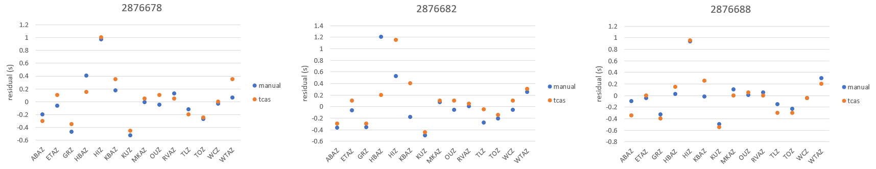
In this post we have shown that the adaptive stacking tcas can reflect pickings done manually. Here we would like to present how tcas may help us in our seismic tomograpy study.
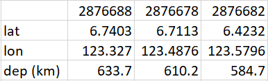
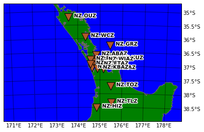
We use a catalog of three events from similar hypocentres travelling to an array of receivers.
-
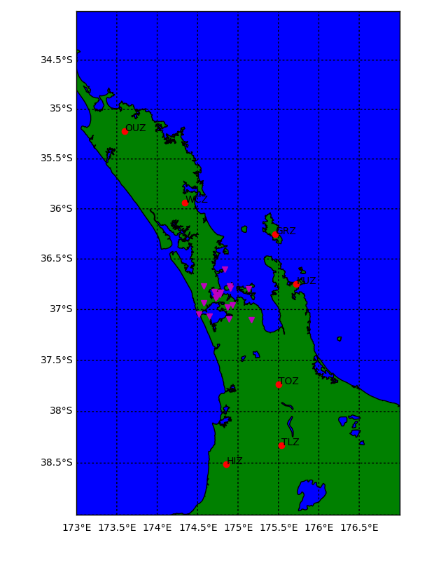
- Receivers
-
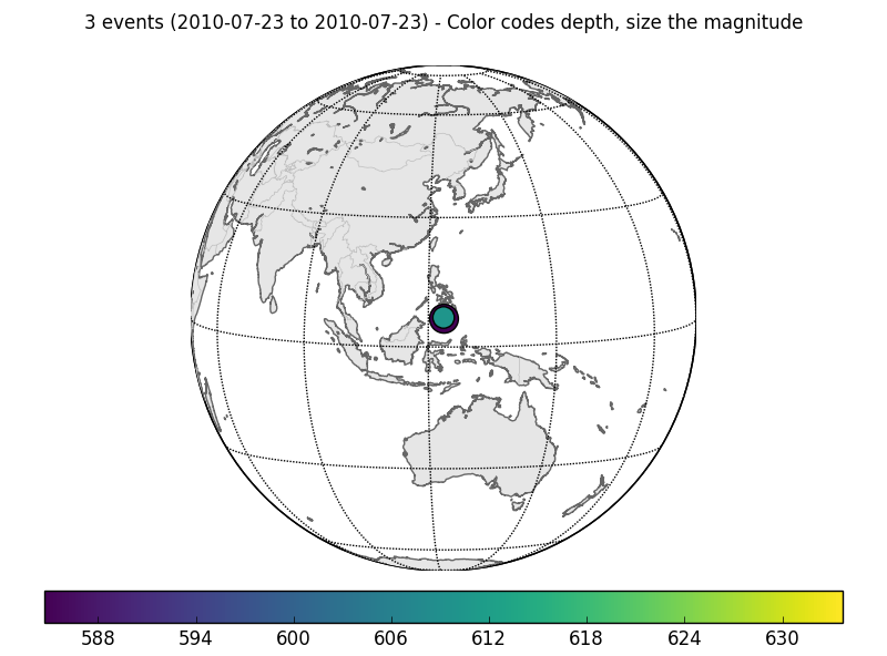
- Events
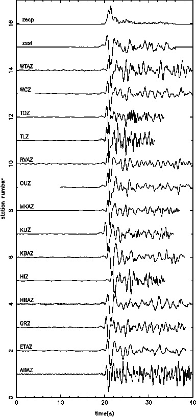
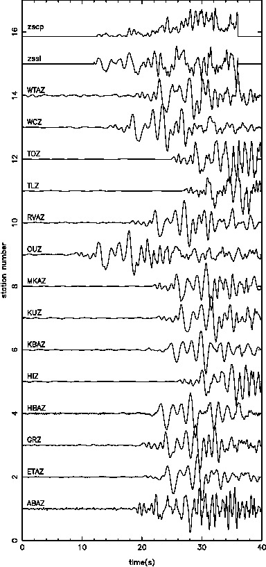
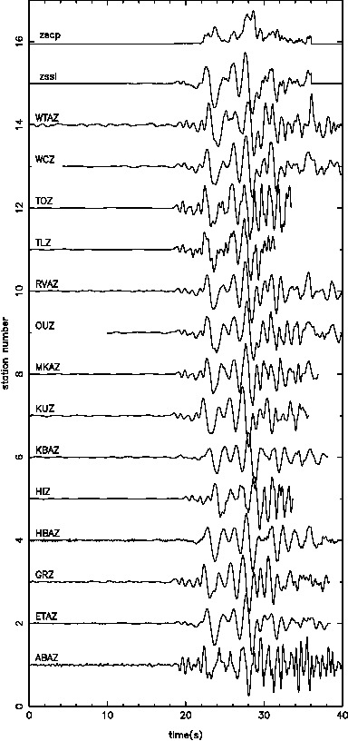
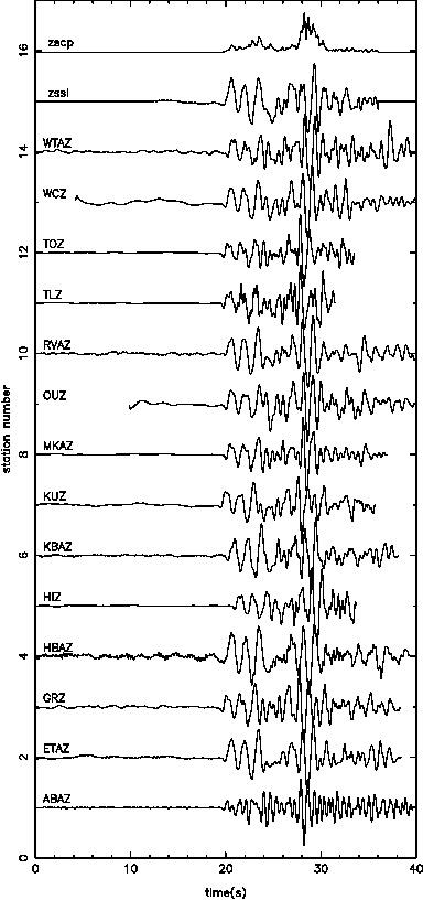
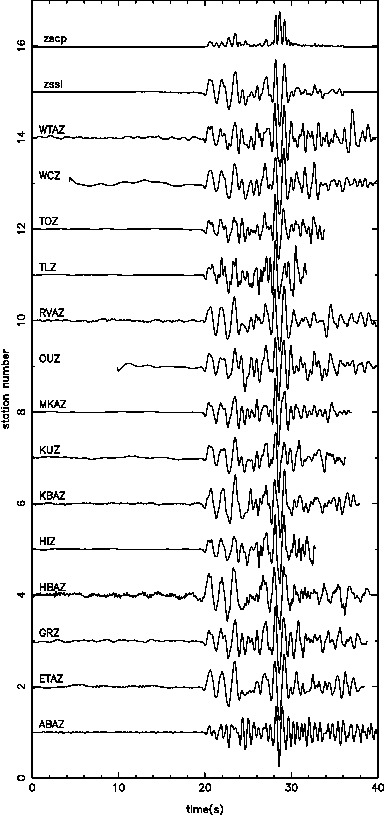
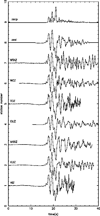
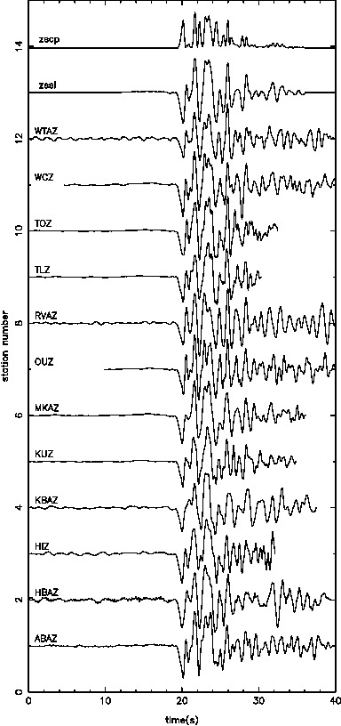
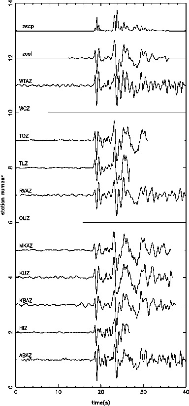
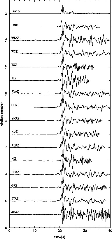
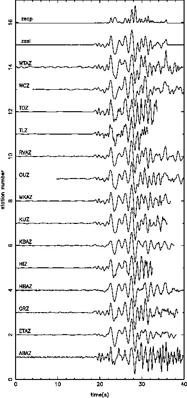
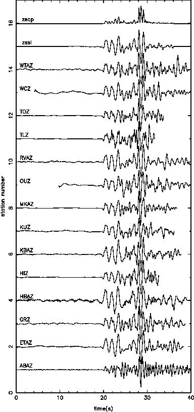
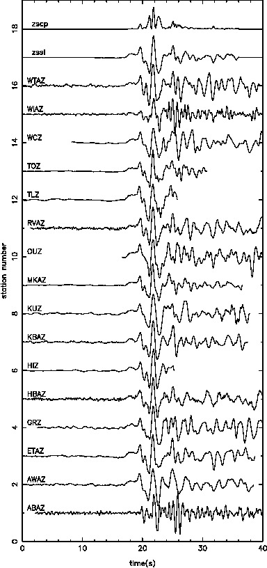
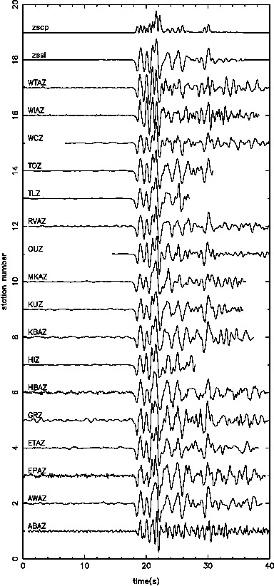
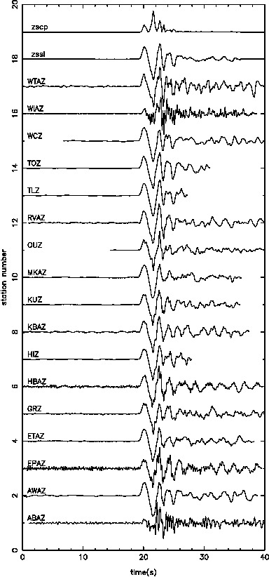
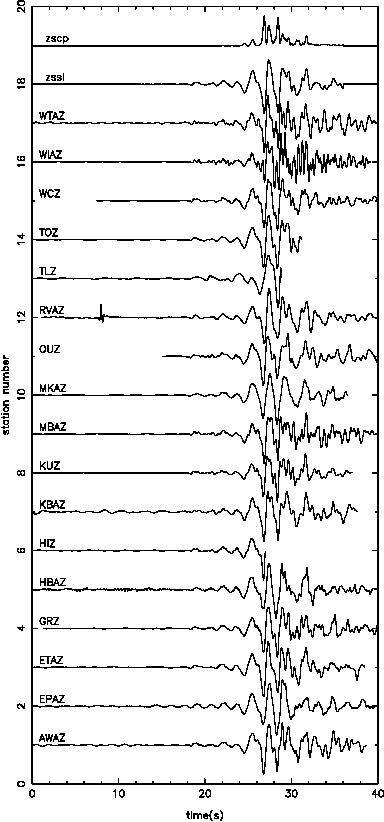
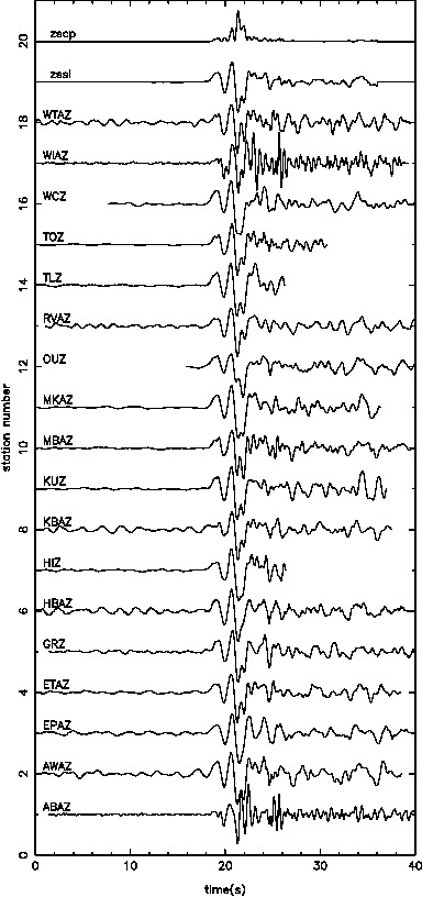
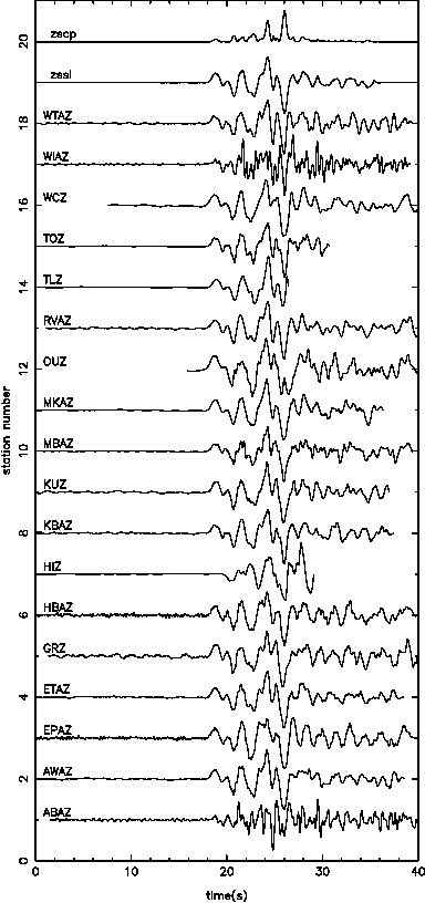
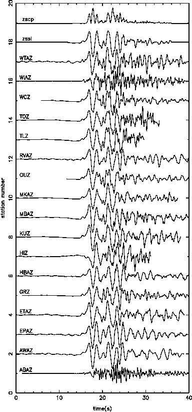
The tcas result shows the following improvement in trace alignment. Each row shows the progression from raw data to initial alignment to the final alignment for one event.
-
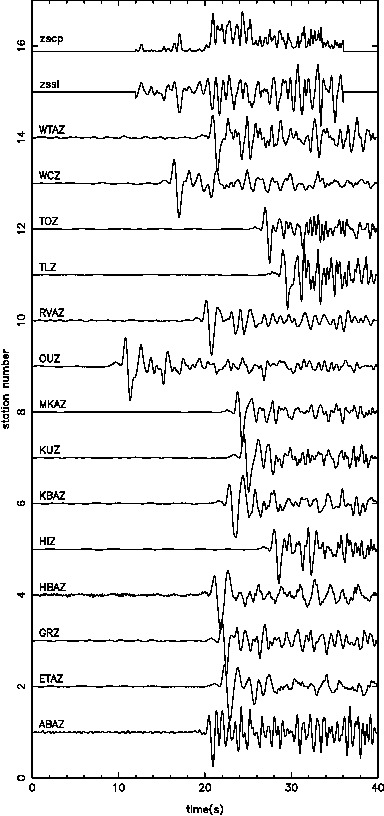
- Raw data
-
- Initial alignment
-

- Final alignment

-
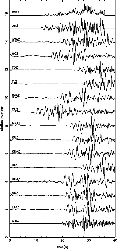
- raw data
-
- initial alignment
-
- final alignment
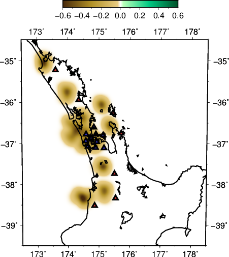
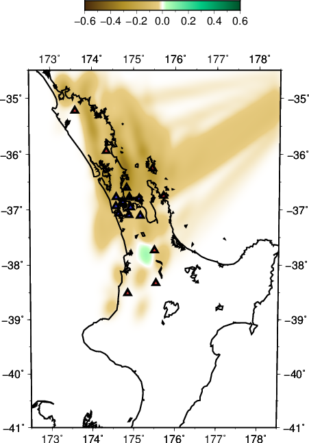
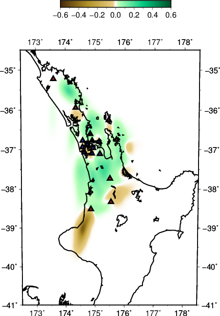
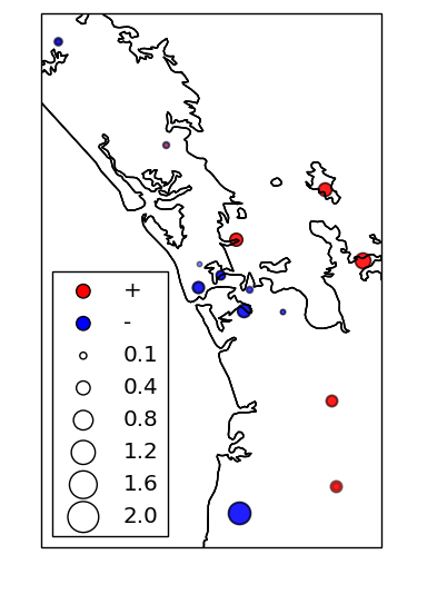
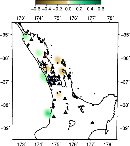
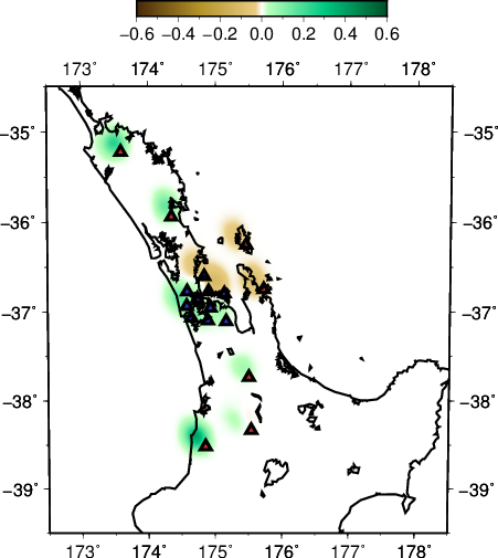
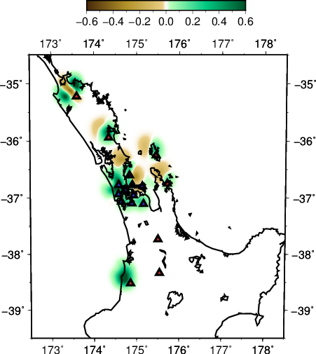
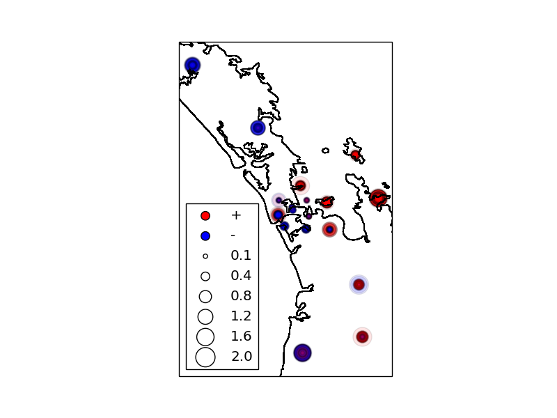
We then plot the residual patterns at every stations that came out from tcas calculation. We superimpose pattern from all events. Red color shows positive residual which means larger than average value thus a slow field and vice versa for blue. The preliminary indication is that we have a slow region to the east of the AVF and fast to the westward.
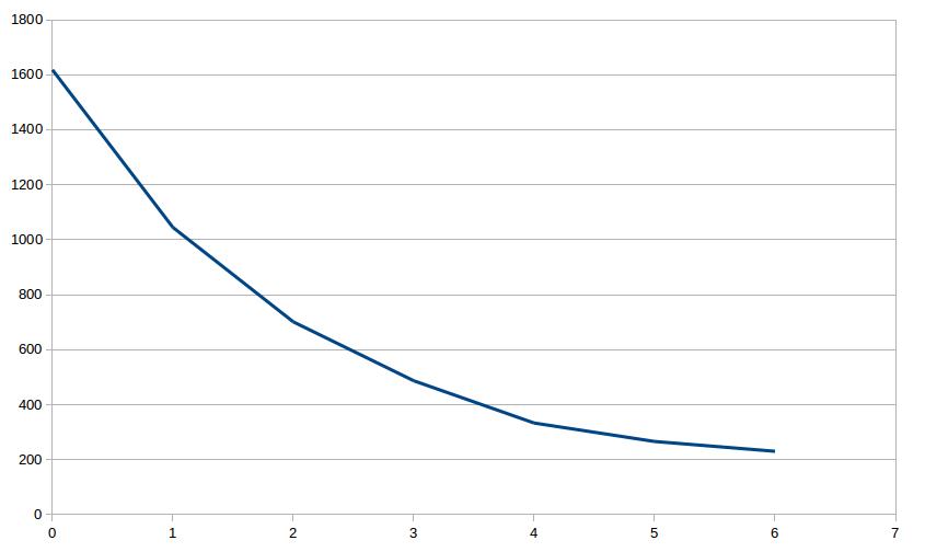
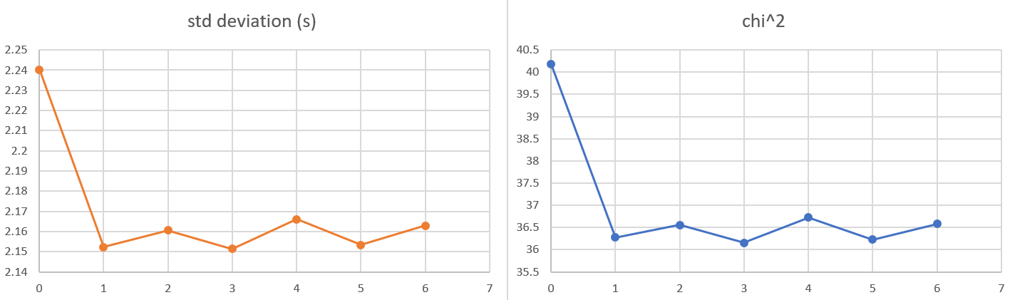
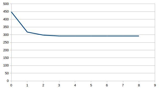
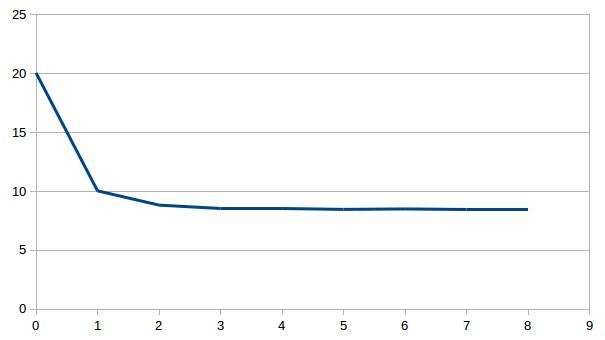
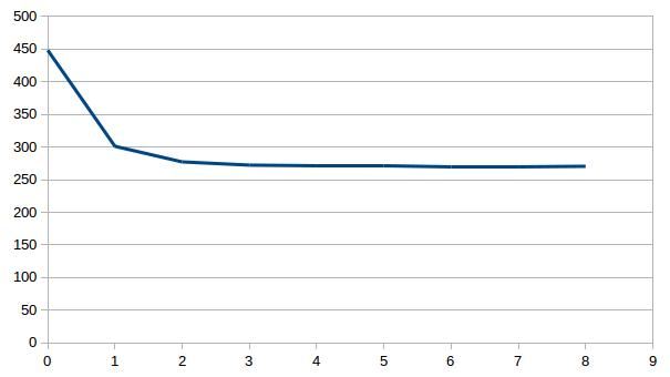
Inversion uses a model with velocity grid cells spread roughly every 0.1 degrees (both NS and EW) and 10 km in depth. The picking error is estimated to be 0.1 s. Regularization is used with damping and smoothing terms of 1 and 2. And we have epsilon equals 1 and eta equals 10. The result shows misfit and chi^2 that are decreasing with iterations. With chi^s converge to value around 1 after two iterations.
-
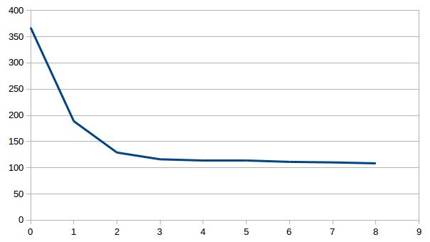
- rms residual (ms) vs iterations
-
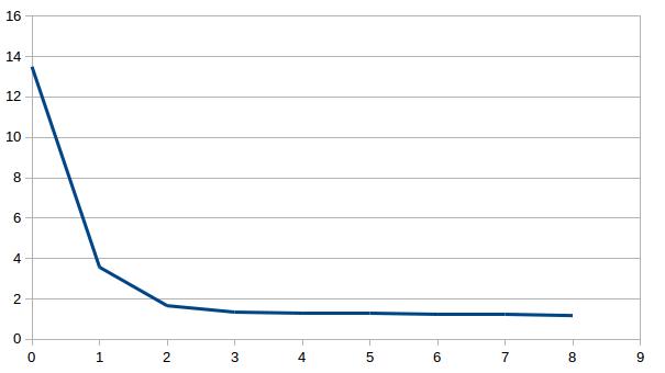
- chi^2 vs iterations
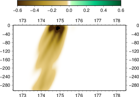
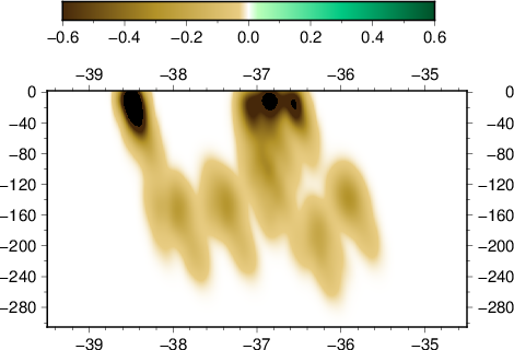
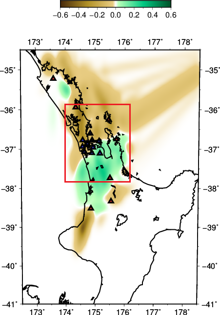
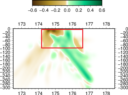
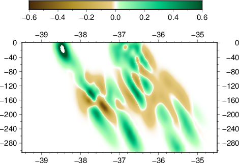
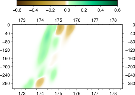
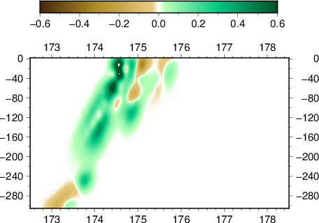
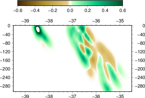
The resulting model presents a perturbation of velocity field around the average with similar pattern to the presumption.
-
- depth slice at 80 km
-
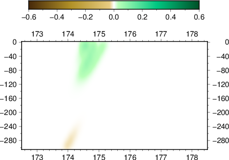
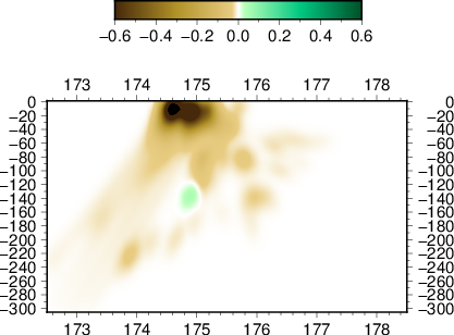
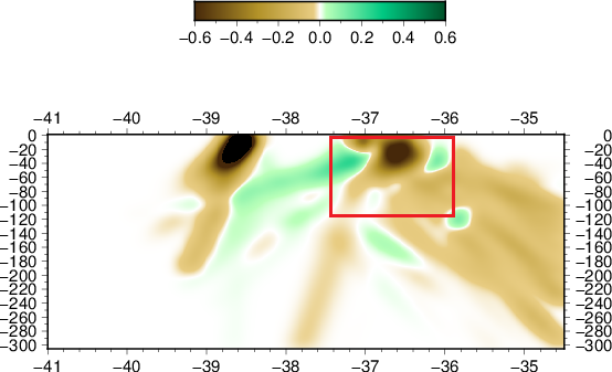
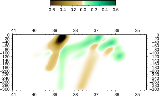
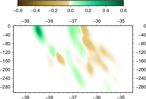
- EW slice at 37.0 S
-

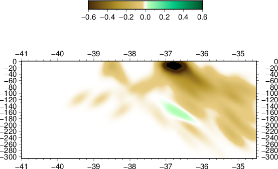
- NS slice at 174.75 E
more events
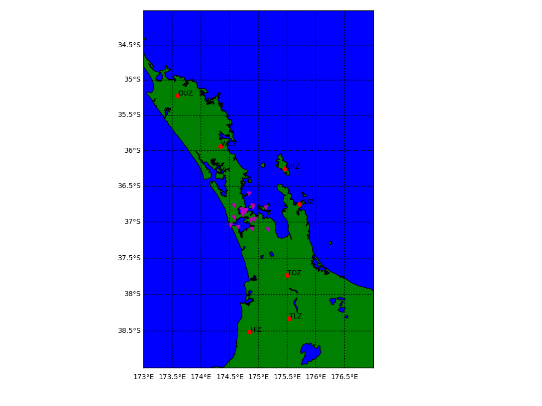
We move forward this time by adding more earthquakes as our sources. As a qualification, we consider teleseismic events further than 27 degrees epicentrally from Auckland. Also we only consider events with good quality data by plotting and judging the trace output. We end up with 13 events.
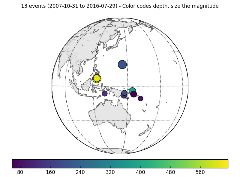
There are reversal in polarity at station HIZ for events prior to 2014, and at OUZ before 2004. This has been addressed prior to applying tcas.
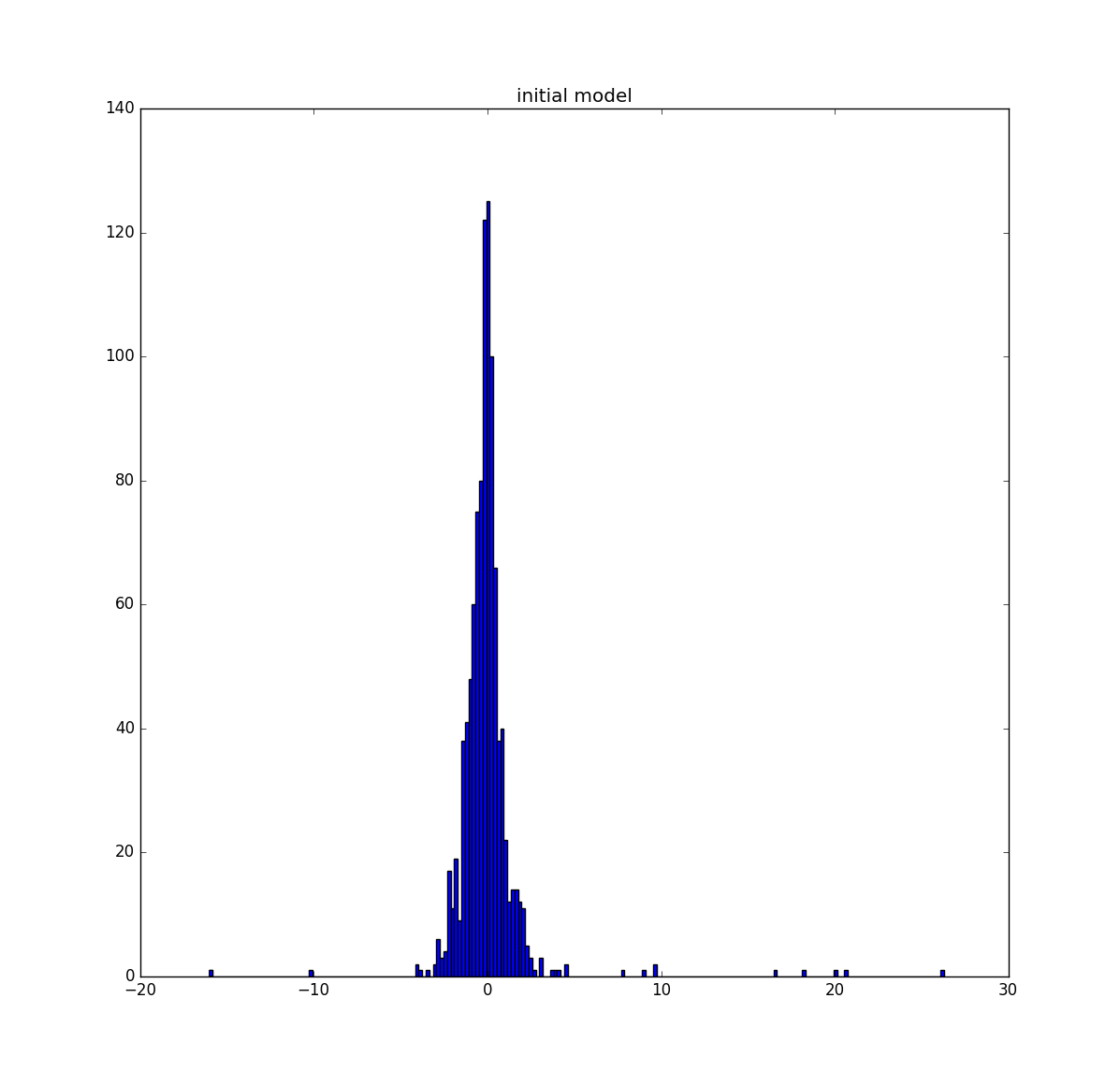
Final tcas alignment for all events shows good results. The output of its residuals/final time-shifts too are well contained between +/- 2 s. So we think tcas has performed as we expect.
The map of the residuals across the array shows more consistency. We again see slow velocity to the east of AVF.

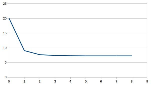
Using the same model, inversion is done with standard deviation set to 0.1 s. If we decide to make all regularization terms equal to 0, chi^2 seems to converge around 7 after 4 iterations. This is equivalent to a variance reduction of 65%.
-
- rms residual (ms) vs iteration
-
- chi^2 vs iteration
-
- depth slice at 35 km
-
- EW slice at 36.75 S
-
- NS slice at 174.75 E
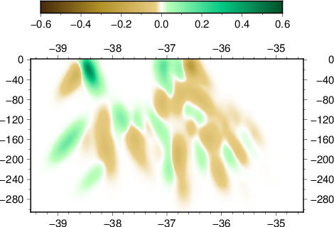
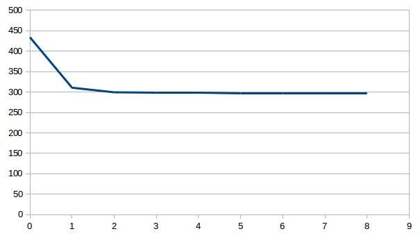
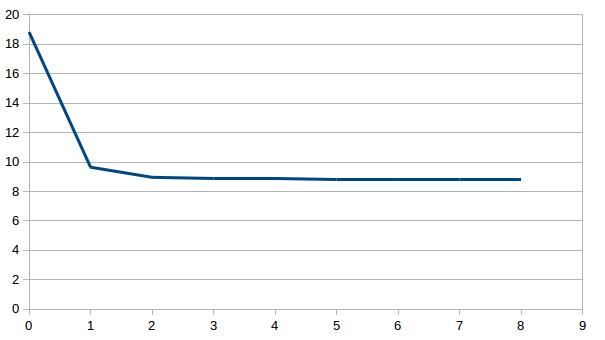
With regularization parameters for damping and smoothing set to 1 and 1 with epsilon of 4 and eta of 8, velocity anomaly start to show a pattern resembling the dt residual map. Chi^2 converge to 8 after 2 iterations.
-
- rms residual (ms) vs iteration
-
- chi^2 vs iteration
-
- depth slice at 35 km
-
- EW slice at 36.75 S
-
- NS slice at 174.75 E
station TLZ and TOZ
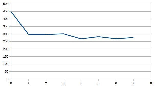
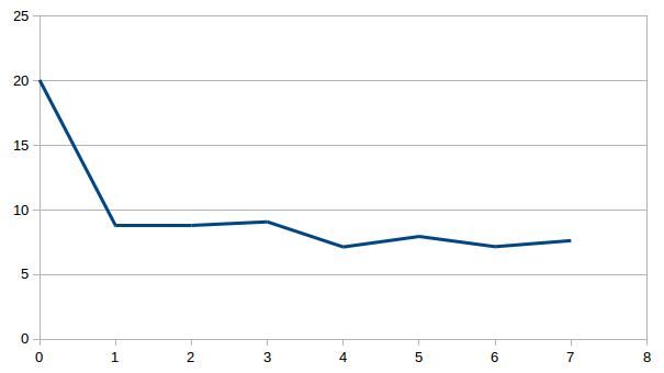
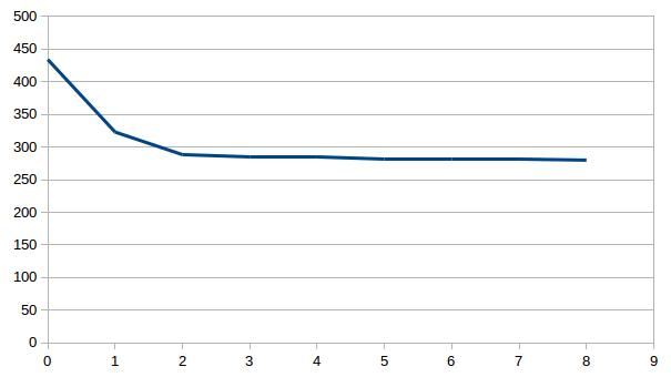
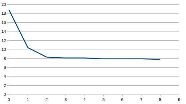
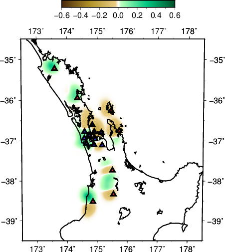
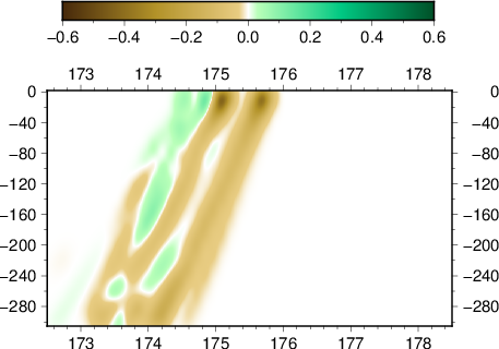
It seems like the conflicting information at station TLZ and TOZ prevent the fit to go below chi^2 equals to 7. Once we removed these two stations from the inversion, chi^2 converge around 5 after 4 iterations with regularization terms set to zero. The variance is reduced from 0.20 to 0.05 s^2 or equal to 75% reduction.
-
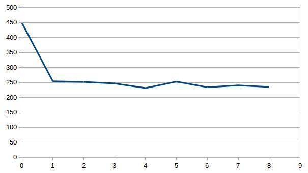
- rms residual (ms) vs iteration
-
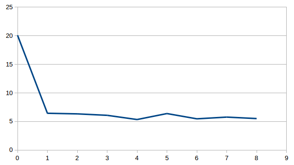
- chi^2 vs iteration
-
- depth slice at 35 km
-
- EW slice at 36.75 S
-
- NS slice at 174.75 E
Similarly with the same regularization applied, chi^2 converge to 7 after 2 iterations but with more coherent resulting model.
-
- rms residual (ms) vs iteration
-
- chi^2 vs iteration
-
- depth slice at 35 km
-

- EW slice at 36.75 S
-
- NS slice at 174.75 E
inversion with catalog of 100+ events
We keep adding events for consideration in the inversion to get a better image of the subsurface presented by the resulting model. We would like to limit our teleseismic event to be not closer than 27 degrees epicentrally from our most Northwesterly station to triplication of arrival. The resulting catalog consist of 166 events:
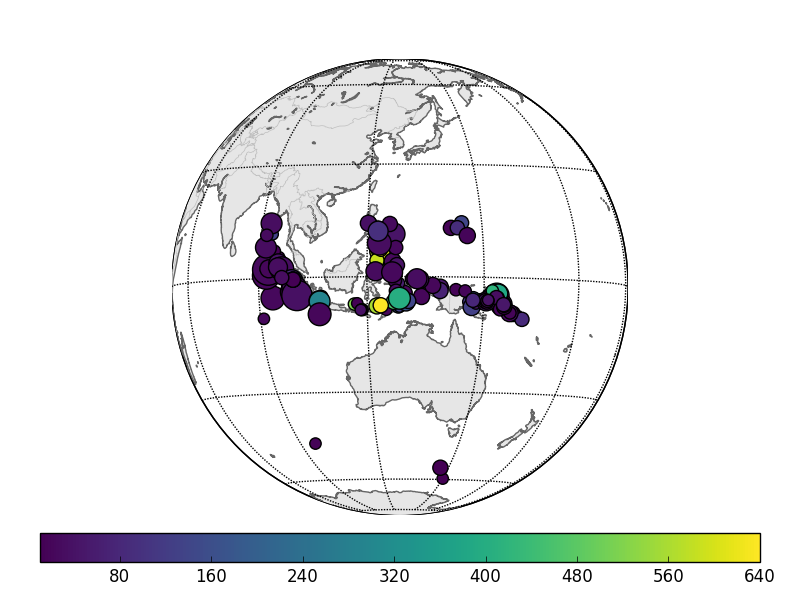
We would also like for the catalog to contain only data with reasonable signal quality after lowpass filtering of 2.0 Hz has been done. On top of data availability, this cut the usable source data further but still we have 131 earthquakes which we have better confidence to work on.
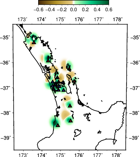
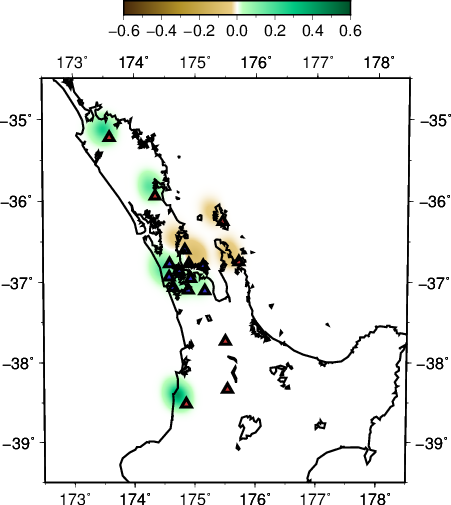
After performing tcas to these events, we plot the residual dt map using the output from tcas. The map shows that the trend of slow to the east of AVF is retained. Residuals at station TLZ and TOZ are more consistent too. There are some stations near the centre where the prevalent residuals can be negative and positive. But these are fairly close to the orientation of the presumed split from fast to slow, so we think this is an understandable outcome.
The output of the inversion with zero regularization shows the following.
-
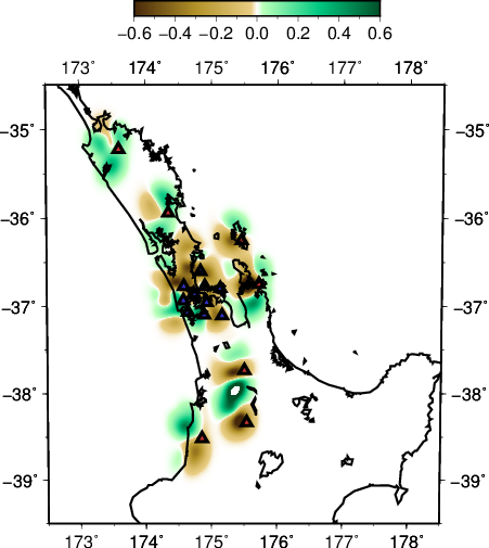
- depth slice at 35 km
-
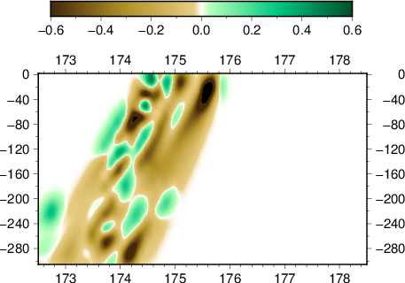
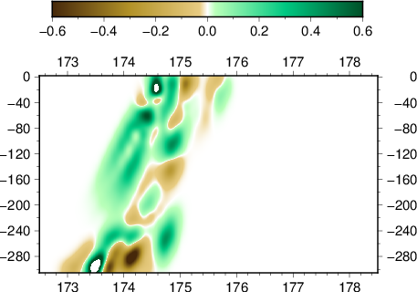
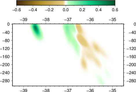
- EW slice at 36.75 S
-
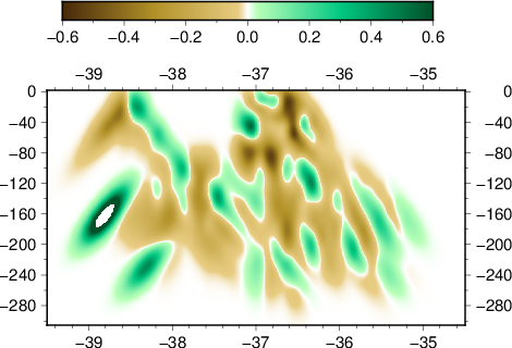
- NS slice at 174.75 E
-
- rms residual (ms) vs iteration
-
- chi^2 vs iteration
While by using the same regularization parameters as the previously,
-
- depth slice at 35 km
-
- EW slice at 36.75 S
-
- NS slice at 174.75 E
-
- rms residual (ms) vs iteration
-
- chi^2 vs iteration