Month: January 2014

Our computing environment

As 21st century researchers, we have access to a tremendous amount of software to practice our trade. In fact, it seems every day new software appears (and some old favourites go out of style, or cease to be supported).  Below is a list of my personal favourites. The common thread here is that these are all open-source software. The reason for this is that open-source software is community supported (and often community-built). There is no messing around with the license files,  there are no black-box results (you have the source code) and even if your institution could afford the commercial programme, maybe your collaborators cannot. Or you can’t run it on your computer at home. By the way, while I shortly will advocate for the linux computer operating system, the software we list is all platform independent.

  • Our operating system of choice is linux. While there is still a bit of a learning curve, installing and learning linux these days is easy. Certainly easier than it was! As is maintenance and upgrading with tools such as apt-get and dnf. There are many flavours of linux, and the differences are really not that great. Within linux, emacs is my personal favorite text editor, but there are plenty of other good ones. Gone are the days of straight-up vi!
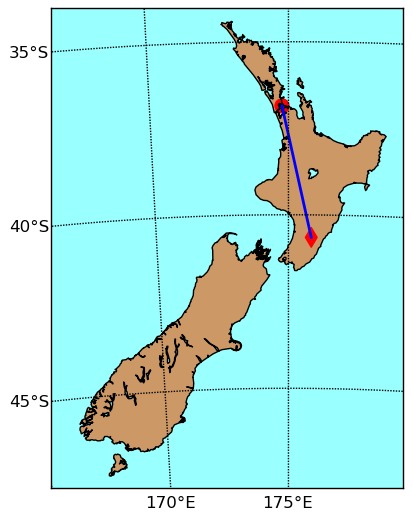
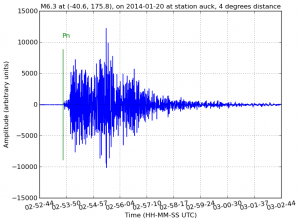
  • Our computer programs are in python, using scipy and numpy. Python is growing so fast that every time I look, there is another new part to python that makes the life of a researcher easier. Processing seismic data was done in SAC or Seismic Unix, but now there is obspy. Making maps without the commercial GIS software required Generic Mapping Tools, but now python with matplotlib, basemap and cartopy ensure vectorised figures and maps. In experiments, we control the hardware in our lab with python. Commercial options such as Labview and matlab are simply obsolete.
  • Document processing is done in LaTeX. You can spot a LaTeX document from a mile away by its beautiful layout, fonts, figures, and maybe most importantly: its equations. Figure labels, section headings, equation numbers are all dynamically linked, making editing a breeze. With only a few lines difference, you can turn a paper into a presentation or a poster, too. Libreoffice, which used to be openoffice, is not bad, but often does not map one-to-one between commercial versions of Word.
  • We draw in inkscape. I love all the vectorized plotting options, and LaTeX implementations with pdf outputs. Wow! Even an awful drawer like me can make something look decent.
  • We tinker with arduino. Projects on school seismometers and a so-called bat-hat for a local museum rely on the wonderful open-hardware that is arduino. We foresee arduinos taking over simple lab tasks in the near future.

Our "seismometers in schools" project received SEG support and is in the news

One of our favourite projects in the Physical Acoustics Lab involves outreach and education in seismology with the TC1 seismometer. This week has been a good week, as we were informed that the Foundation of the Society of Exploration Geophysicists (SEG) will support the instrumentation of a number of NZ schools with seismometers. In addition, Ian Randall wrote a wonderful article on the topic in Physics World.

M6.3 earthquake, 15 km east of Eketahuna

greatcircle

 
In the Science Centre of the City Campus of the University of Auckland we record seismic waves with the TC1 seismometer. Routinely, our station AUCK records seismic waves from earthquakes in New Zealand and beyond. On January 20th, 2014, an earthquake occurred on the South side of the North Island, 15 km east of Ekatahuna. Here is a map of the epicentre, our station location, and the great-circle path between them.


2014-01-20-02-52-44

On the left you can see 10 minutes of recordings, starting at the origin time of this earthquake. The green marker annotated with a Pn is the predicted arrival of the first wave traveling 4 degrees from the epicentre, 15 km east of Eketahuna, to Auckland. This prediction is based on a spherically symmetric model of the Earth, by Brian Kennett, and certainly seems to mark the start of minutes of vibrations in Auckland from this earthquake. In fact, if you look carefully you see that the wiggles after 10 minutes are still larger than before the first wave from this earthquake arrived. Larger earthquakes can make the Earth “ring” for many hours.

2014-01-20-02-52-44_zoom
In the image on the right, we zoomed in on the first-arriving wave, almost exactly one minute after the earthquake originated. Now, you can see that the prediction is actually a few seconds before the arrival. This means the lithosphere under the North Island of New Zealand is a bit slower (~3% on this path) than the average on Earth. In general, a hotter lithosphere is slower than a cold one. This makes seismic waves traversing old, cold, continents relatively fast, and those sampling younger lithosphere like ours in New Zealand, relatively slow.

In general, it is these small travel time differences that provide images of the (deep) earth through a process called seismic tomography.

Our paper on photoacoustics came out

Today, the manuscript based on Jami Johnson’s research in medical imaging with photo-acoustic waves came out. Congratulations, Jami! You can find the paper here. For a complete list of the publications of members of the Physical acoustics lab, including pdf reprints, visit our pubs page